Breaking Down a RAG Pipeline: Where Latency Really Comes From

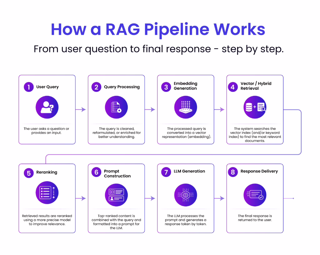
Most teams assume the LLM is the main reason their RAG system feels slow. But in production, latency rarely comes from just one place. The real delay hides across multiple layers such as retrieval, reranking, network hops, prompt assembly, token generation, and orchestration logic, each quietly adding up before a single word reaches your user.
And while generation is often the largest single contributor, retrieval-side overhead compounds fast the moment you introduce multi-stage search and reranking. To optimize RAG performance, you first need to understand where every millisecond is going.

What a Typical RAG Pipeline Looks Like

To optimize RAG performance, you first need to understand where every millisecond is going.

Where Latency Actually Comes From

At a glance, a RAG pipeline feels like a clean, linear flow. In reality, latency builds up in layers, small delays at each stage that compound into noticeable response time. To optimize effectively, you need to understand where those milliseconds are really being spent.

Embedding Latency: Small but Non-Zero

Embedding models are relatively fast but not free. Each query must be converted into a vector before retrieval can even begin. Under light usage, this feels negligible. At scale, or with larger embedding models, this step can introduce consistent overhead, especially if requests are not batched or cached. Network calls to external embedding APIs can further amplify this delay.

Retrieval Latency: Data Size Matters

Vector or hybrid search is often assumed to be instant, but performance depends heavily on index size, query complexity, and infrastructure. Searching across millions (or billions) of vectors requires optimized indexing. Poorly tuned databases, cold caches or distributed queries can all add tens to hundreds of milliseconds here.

Reranking Overhead: Accuracy vs Speed Trade-off

Reranking improves relevance, but it comes at a cost. Each retrieved document (often top 10–50) may be passed through a secondary model to score relevance more precisely. This introduces additional inference time, and unlike retrieval, it scales linearly with the number of candidates. The better quality you want, the more latency you’re likely to pay.

Prompt Construction: The Hidden Multiplier

This step is frequently underestimated. Combining retrieved chunks with the query isn’t just string concatenation, it involves formatting, deduplication, truncation and token budgeting. Inefficient prompt construction can inflate token count, which directly impacts LLM processing time. More context is not equal to better performance if it slows everything down.

LLM Generation: The Primary Bottleneck

This is where most of the latency lives. Large language models generate responses token by token, and the time taken depends on:

• Model size (larger models = slower inference)
• Output length (more tokens = more time)
• Hardware and serving setup (GPU vs CPU, batching, etc.)

Even a well-optimized upstream pipeline can feel slow if generation isn’t controlled. This is why techniques like streaming responses, output limits, and smaller models are often used to manage perceived latency.

Network & Orchestration Overhead: Death by a Thousand Cuts

Each stage in the pipeline often involves separate services, embedding APIs, vector databases, rerankers, LLM endpoints. Every hop introduces network latency, serialization/deserialization time, and orchestration overhead. Individually small, collectively significant.

Cache Misses: The Silent Latency Killer

Caching, whether for embeddings, retrieval results, or final responses can dramatically reduce latency. But when caches miss (which they often do for dynamic queries), the full pipeline executes. Systems without intelligent caching strategies end up paying the full latency cost repeatedly.

The Hidden Multipliers: Why Latency Grows Faster Than You Think

At a glance, each stage in a RAG pipeline adds a small delay. In practice, latency compounds. Small decisions early in the pipeline increase the cost of every step that follows, especially LLM generation.

The Hidden Multiplier

Prompt assembly is often underestimated. Every extra 100 tokens added to the prompt doesn’t just affect formatting, it directly increases LLM workload.

More tokens mean:

• Higher time to first token (TTFT)
• Longer generation time

Since the model must process all input tokens before generating a response, even small increases in context size amplify latency in the most expensive stage.

The Context Tax

Adding more chunks during retrieval introduces a cascading cost:

• More documents to rerank
• Larger prompts to construct

Slower LLM generation due to increased context

Because LLMs scale poorly with larger inputs, a few extra chunks can lead to a disproportionate increase in total latency.

More context isn’t always better. Beyond a point, it just makes the system slower.

Latency is Multiplicative

RAG latency isn’t the sum of independent steps. Each stage expands the workload for the next.

What looks efficient in isolation can still feel slow in production, because small inefficiencies multiply across the pipeline.

What Actually Happens Inside a RAG Pipeline

1) Query Preprocessing & Embedding

Before retrieval begins, the system first prepares the query for semantic search. This includes basic text cleaning to normalize the input, followed by query rewriting in some cases to improve clarity or expand intent. The refined query is then passed through an embedding model to generate a vector representation, which becomes the foundation for retrieval. Alongside this, any metadata filters, such as time range, document type, or user-specific constraints are attached to guide more precise results.

Typical latency: 20–100 ms

This stage is usually quick and predictable. However, if embedding generation relies on external APIs, network calls can introduce additional overhead, making this step slightly more noticeable at scale.

2) Retrieval Layer

This is the stage where latency starts to become more noticeable and often underestimated. Once the query embedding is generated, the system moves into retrieval, where it searches for the most relevant pieces of information. This typically involves vector search to capture semantic similarity, often combined with BM25 or hybrid retrieval to ensure keyword-level precision. At the same time, metadata filtering is applied to narrow down results based on constraints like source, time, or access level.

Under the hood, the system is querying a large index of stored embeddings and documents, and performance here depends heavily on how that index is structured and accessed. While modern vector databases are optimized for speed, retrieval is not always “instant” especially as the dataset grows.

Typical latency: 10 – 150 ms

For smaller corpora, this step is fast and predictable. However, as the data scales, latency increases due to several factors:

• Index size: Larger datasets require more work to search efficiently
• ANN search strategy: Faster methods may trade accuracy for speed, while more precise searches take longer
• Distributed infrastructure: In multi-node or cross-region setups, network latency between nodes can dominate the total time

In many real-world deployments, this stage becomes a key contributor to overall latency, not because any single operation is slow, but because of the combined cost of searching, filtering, and moving data across systems.

3) Reranking (Often Hidden Latency)

Reranking is where the system refines its initial results but it’s also one of the most overlooked sources of delay. After retrieval, you might have the top 20–50 candidate chunks. A cross-encoder reranker then evaluates each query, document pair more precisely, scoring them for true relevance. This allows the system to narrow results down, for example, from top 50 to top 5 before passing them to the LLM.

Unlike vector search, which is optimized for speed, reranking involves deeper computation. Each candidate is processed individually, which means latency scales with the number of retrieved chunks. The more you want accuracy, the more time this step tends to take.

Typical latency: 80 – 300 ms

This step significantly improves answer quality and reduces irrelevant context, but it comes at a cost. In many pipelines, reranking quietly becomes a major contributor to overall latency.

Ironically, the step added to improve relevance is often the step that slows the experience the most.

4) Prompt Assembly

This is one of the most underestimated parts of the pipeline. After retrieval and reranking, the system has to turn raw results into a structured prompt that the LLM can actually use and that process isn’t just simple concatenation.

It starts with merging the retrieved chunks, often cleaning, deduplicating, and ordering them for coherence. Then comes citation formatting, where sources are tagged or structured so the final response can reference them correctly. On top of that, the system injects system prompts or instructions, guidelines that control tone, behavior or output format. Finally, there’s token counting and budgeting, ensuring the entire prompt stays within model limits while still preserving the most useful context.

Typical latency: 20 – 80 ms

Individually, these operations are lightweight, but they add up, especially as the amount of context grows. Latency can rise quickly when:

• Too many chunks are included
• Context windows become large
• Prompt templates become complex or heavily structured

This stage often flies under the radar, but inefficient prompt assembly can inflate token usage and directly increase the time spent in the most expensive step: LLM generation.

5) LLM Generation

This is the heart of the pipeline and almost always the biggest contributor to latency. No matter how optimized the earlier stages are, the moment the request hits the LLM, response time becomes heavily dependent on model behavior and output size.

Typical latency: 500 ms to 5+ seconds

For most real-time systems, this stage dominates overall latency. Even small inefficiencies upstream can amplify delays here because the model processes everything token by token.

To understand where the time goes, it helps to break this step down further:

• Time to First Token (TTFT): This is the delay before the model starts generating anything. It includes prompt processing, model loading, and initial computation. A slow TTFT makes the system feel unresponsive, even if generation speed is decent afterward.
• Token Generation Speed: Once generation starts, the model produces tokens sequentially. Speed depends on model size, hardware, and optimization. Larger models tend to be slower but more capable.
• Long-Form Answers: The more tokens you generate, the longer it takes, simple as that. Verbose responses or unbounded outputs can quickly push latency into multiple seconds.
• Reasoning-Heavy Models: More advanced models (especially those optimized for reasoning or chain-of-thought tasks) often take longer per token. The trade-off is better quality, but at a noticeable cost in speed.

Common Production Mistakes That Increase Latency

Even well-designed RAG pipelines can feel slow in production not because of one major flaw, but due to a series of small decisions that quietly add up. These are some of the most common culprits:

• Retrieving too many chunks: Pulling excessive context increases reranking time, bloats the prompt, and slows down generation.
• Multiple reranking passes: Stacking rerankers might improve accuracy slightly, but it compounds latency quickly.
• Cross-region infrastructure: When components (LLM, vector DB, APIs) are deployed in different regions, network round trips add significant delay.
• Slow or poorly tuned vector databases: Inefficient indexing or suboptimal ANN configurations can make retrieval slower than expected.
• No caching strategy: Without caching embeddings, retrieval results, or responses, the system repeatedly pays the full latency cost.
• Overly long prompts: More tokens mean longer processing and generation time, often without proportional quality gains.
• Using oversized models by default: Larger models improve quality, but using them for every request can drastically slow down response times.

How to Reduce Latency in a Production RAG Stack

Reducing latency isn’t about one silver bullet, it’s about tightening each stage of the pipeline and eliminating unnecessary work. The most effective systems focus on doing less, smarter.

Retrieval

Start by optimizing how much and how fast you fetch:

• HNSW / IVF optimization: Tune index parameters to balance recall and speed based on your dataset size
• Hybrid search tuning: Adjust vector vs keyword weighting to avoid redundant or noisy results
• Reduce top-k: Fetch fewer chunks upfront to cut down reranking cost and prompt size

Generation

This is where most latency lives, so even small changes matter:

• Smaller serving models: Use the smallest model that meets quality needs instead of defaulting to the largest
• Response streaming: Improves perceived speed by reducing time to first token
• Answer templates: Structured outputs reduce token usage and generation time

System

System-level design decisions often have the biggest compound impact:

• Semantic caching: Cache embeddings, retrieval results, or full responses for repeated queries
• Async retrieval: Parallelize steps where possible instead of waiting sequentially
• Batching: Group requests to improve throughput, especially for embeddings and reranking
• Colocated infrastructure: Keep services in the same region to minimize network latency

Wrapping Up

RAG latency isn’t just about the model, it’s the sum of every step in the pipeline. Small delays in retrieval, reranking, prompt assembly, and network hops quietly add up to shape the final experience. The fastest systems aren’t the most complex, they’re the most intentional, doing less but doing it smarter. By measuring each stage and eliminating unnecessary work, you can significantly improve performance without sacrificing quality.

Start by breaking down your pipeline, identifying where time is spent, and optimizing one step at a time. Because in production, speed is not a feature, it’s a design decision.